Steady Storage Stampede

PG Phriday: Steady Storage Stampede
When we are sizing our database storage, we don’t always take performance metrics such as operations per second into consideration. A direct consequence of this may be that we won’t attain the performance we’re seeking. Yet there’s a more insidious side-effect here that’s buried deep in the bowels of the operating system itself: memory flushing.
In an age where SSD and NVMe devices are readily available from all cloud providers and reasonably priced for bare metal servers, it’s easy to forget the effects of write caching. These devices can easily absorb tens of thousands of operations per second, after all! Rather than flushing data to an intermediate storage controller cache, we can effectively write directly to the device itself because it’s so fast.
But what actually happens when we overwhelm our SSD or NVMe devices? Is this even possible for such high performance devices?
A Bit of Background
While performing some benchmarks related to an internal project here at EDB, we noticed some particularly odd behavior. Performance would actually remain fairly unremarkable for the first few minutes of benchmarks, and then fall precipitously off of a cliff and never recover. Instead of an average of say, 1700 TPS on pgbench, it would end up as 800.
What confused us in these circumstances, is that we didn’t observe the same behavior on our bare metal hardware in our local datacenter. Rather, the precarious drop in throughput happened on a small army of Amazon c5ad.4xlarge instances with marked regularity. Even Amazon’s relatively low performance general purpose volumes are equipped with SSD-equivalent hardware, with a 500GB allocation starting at 1500 IOPS.
Why then, would a standard Postgres benchmark like pgbench provide reasonably good performance, quickly followed by something less savory? Unlike SSDs for the most part, server hard drives are often hidden behind a sophisticated storage controller equipped with advanced RAID and cache functionality. We’ve known for a while that traditional hard disks carry strong performance penalties tied to their geometry and the limitations of physics. In an effort to mitigate the impact of this, these disk controllers may provide several GB of RAM to buffer writes to the ancient spinning rust technology.
SSDs on the other hand, aren’t always so well equipped. They’re so fast, we’ve all but forgotten the concept of a write cache at the controller level, and simply blast the device with writes whether or not it’s capable of absorbing them. Usually the maximum extent to which an SSD carries a cache, are a few paltry super-capacitor-backed memory chips purely to overcome the effects of write amplification inherent to NAND-flash cells. This only protects writes which are in-flight and have not yet committed to the actual memory cells, leaving all pending OS-level write flushes to fend for themselves.
With this knowledge in mind, we decided to see just how well AWS EBS storage fared with various Postgres workloads.
Initial Impressions
We started with the hardware that piqued our interest: a c5ad.4xlarge EC2 instance equipped with 500GB of EBS gp2 allocated at the default of 1500 IOPS with up to 3000 IOPS burst performance. For the uninitiated, a c5ad.4xlarge provides 16 AMD EPYC CPU threads and 32GB of RAM. Then we included a dedicated c5.xlarge (4 CPUs, 8GB RAM) driver system to decouple the benchmark software from the instance being tested.
We bootstrapped these systems with a 10,000 scale pgbench database, equivalent to about 150GB of data, and ran all tests with 32 concurrent clients. To isolate as much as possible, we increased max_wal_size to 32GB to prevent a checkpoint in the middle of a test and increased checkpoint_timeout to 15 minutes so our 500-second tests could run undisturbed. We also moved the pg_wal directory to one of the 300GB local storage devices on the server. This allows measuring read and write performance of the pgbench data itself. This is principally random IO, which would otherwise be disrupted by the sequential write access-path of WAL traffic.
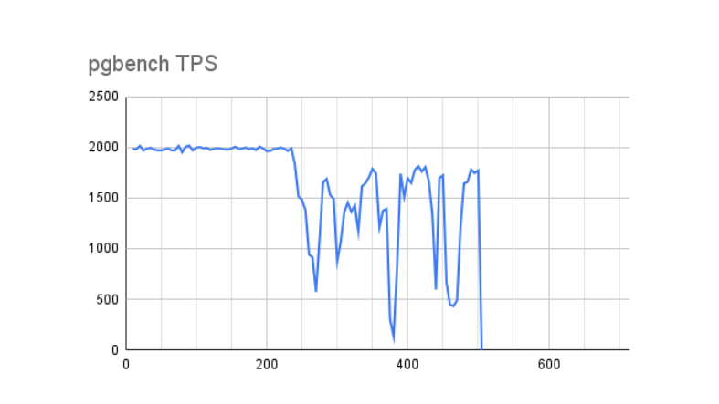
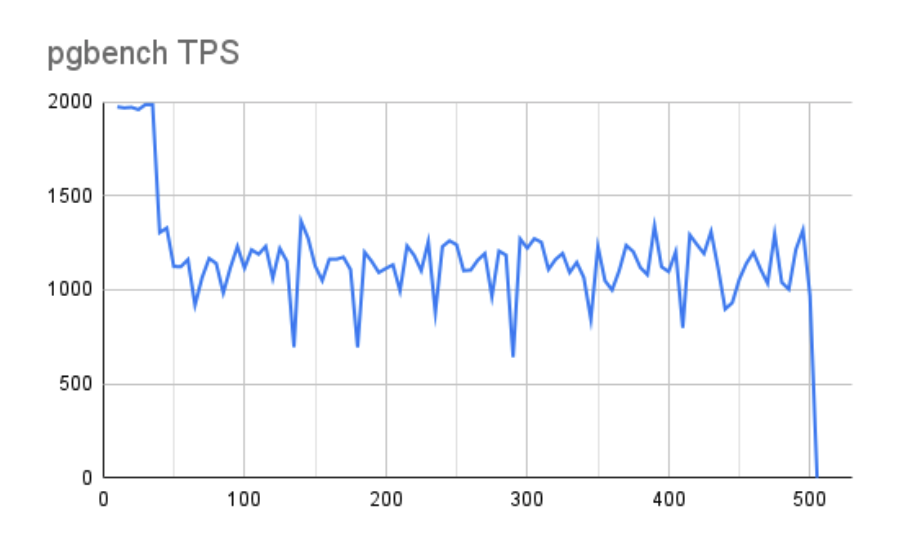
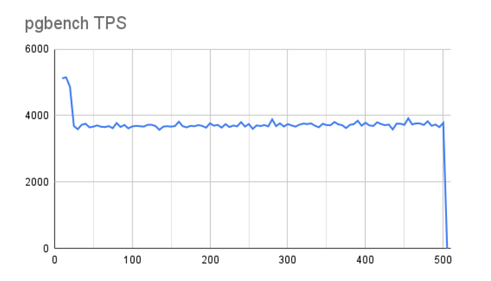
Once we ran the benchmark and tabulated the results, the source of the problem became clear. This first chart outlines pgbench TPS mapped over 500 seconds.
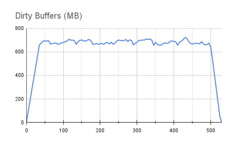
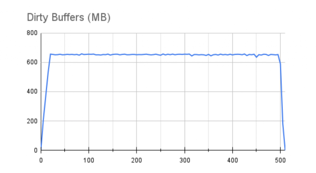
This next chart shows the size of the Linux Dirty Buffer RAM allocation over the same period:
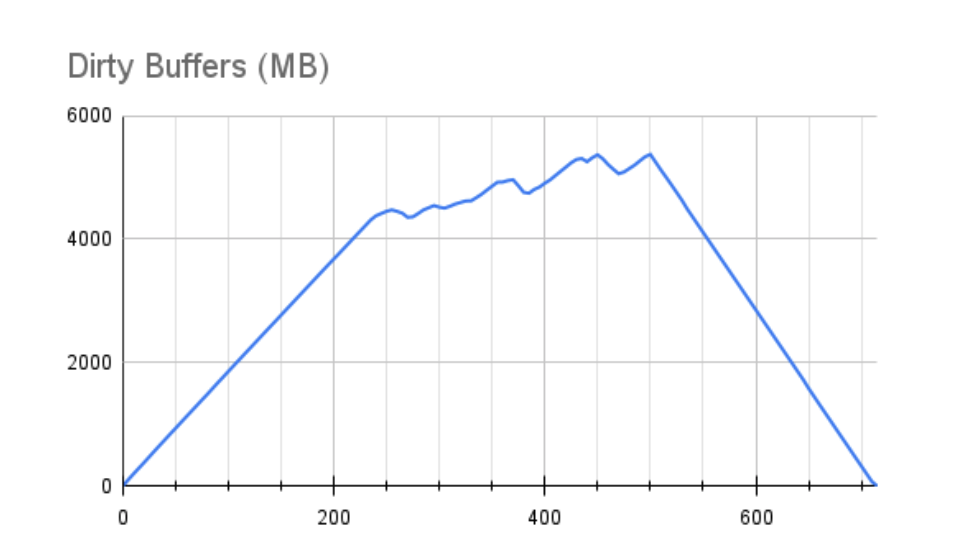
Notice that performance drops right after Dirty Buffers reaches about 4.5GB. On our 32GB server, the range of memory on this chart accounts for roughly 15-20% of available RAM. For those familiar with Linux VM tunables, this behavior is driven by the vm.dirty_ratio kernel parameter, which is often set between 10-20%, but can be higher in many cases.
When Dirty Buffers eclipse the amount of RAM dictated by vm.dirty_ratio, Linux essentially goes sequential, pausing all pending writes to allow the write queue to drain under the ratio. Both charts reflect performance never again reaching its peak, with multiple substantial drops that nearly reach zero TPS over the course of the test. Even after the test ended, the buffers weren’t fully drained for an additional 215 seconds. Keep in mind that many of these buffers may be fsync operations, and indeed our Postgres logs show some checkpoint sync operations required 8-12 seconds to process. What would have happened if we experienced a server hardware failure at this time?
Pushing the Limits
Our standard tuning recommendations reduce vm.dirty_ratio to 10% or lower specifically to prevent long buffer flushes. Indeed, on a server with 512GB of RAM, we probably don’t want 50GB of buffers to start flushing and overwhelm the underlying storage. But there’s still the potential argument that we should increase the maximum dirty buffers to preserve performance.
To give a little more control to the situation, we chose to leverage the vm.dirty_bytes setting rather than vm.dirty_ratio, so we could specify an exact amount of bytes rather than a percentage of RAM. We also constrained the related vm.dirty_background_bytes to 25% of our selected vm.dirty_ratio value to encourage background writes long before reaching that maximum.
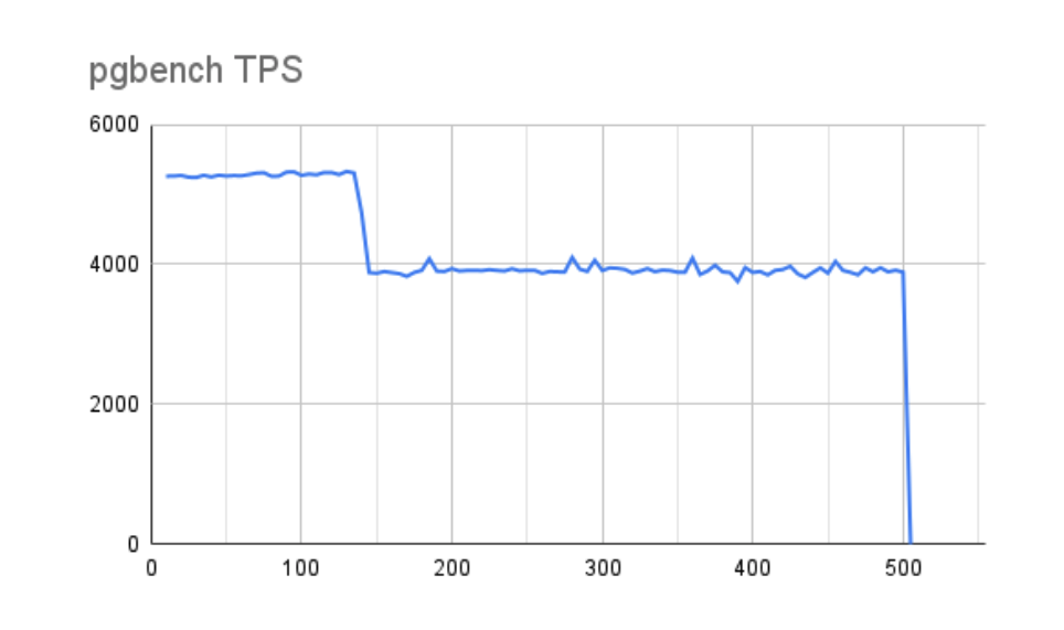
In this next case, we tested with a setting reflecting 16GB of dirty RAM, and ended up with these results:
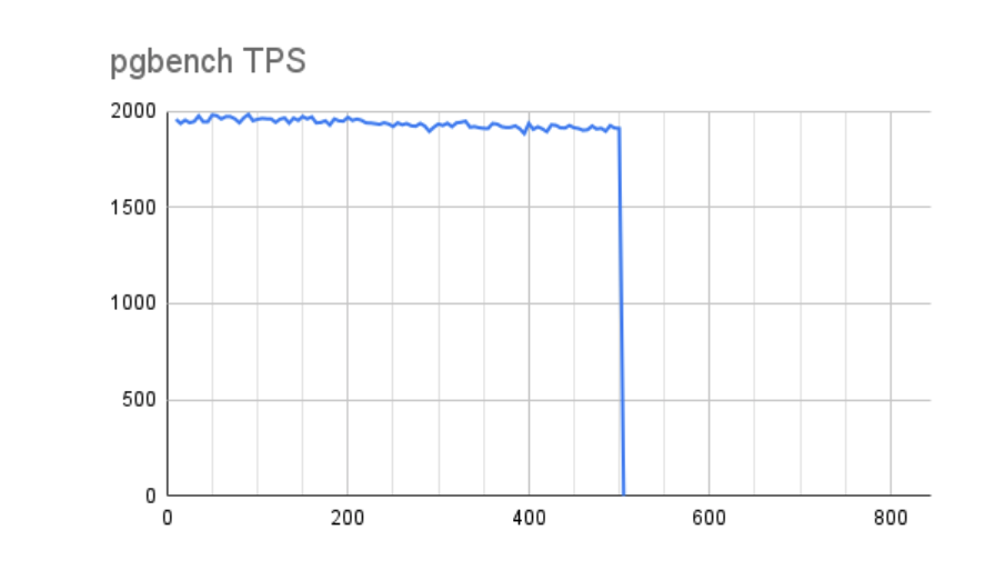
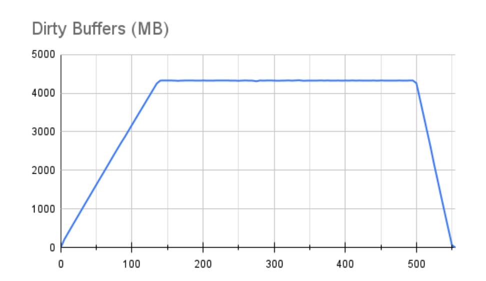
Well that certainly looks like a marked improvement! There’s a slow degradation in performance over time, but nothing substantial. But let’s look at the buffers:
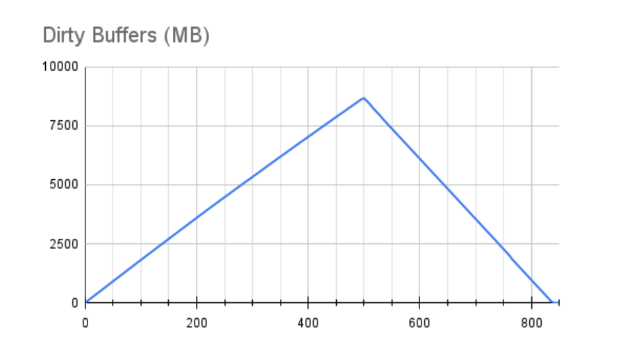
Unfortunately this isn’t nearly as encouraging. The only reason we didn’t see the same drop in performance is because we only reached 8GB of our 16GB total available dirty buffers. Had we allowed the test to run for a longer duration, it would closely resemble the first results, but with a longer x-axis representing our maximum performance. We also can’t ignore that draining these buffers required 345 seconds!
Note: None of these tests modified the default vm.dirty_expire_centisecs or vm.dirty_writeback_centisecs kernel parameters. We attempted various values here and nothing appeared to notably affect the results. Given that the underlying storage device appeared to be fully saturated during these tests, this is expected, as minor tweaks to memory retention periods would not significantly reduce this write volume.
Introducing A Buffer Throttle
It’s a rare condition where we’d prefer throughput over write durability, so what happens if we reduce the maximum size of our dirty buffers? We commonly recommend sizing vm.dirty_bytes to the total size of the storage write cache, if known. Since SSD and NVMe devices don’t tend to have those, we used a low value of 1GB instead.
Our graphs looked a bit different this time around. First, our TPS performance:
While we overflow the 1GB buffer fairly quickly, our performance stalls aren’t quite as pronounced. We can see why this might be the case in the buffer graph:
Perhaps most importantly, a 1GB buffer only required 30 seconds to drain after the test ended. In all of these cases, our tradeoff must always include the fact that dirty writes will continue to accumulate using this storage backend, because of two factors:
- We are overwhelming the underlying storage with write requests.
- There is not sufficient storage caching to absorb this write throughput.
Despite the older and slower performance of the underlying hard-disk drives, a storage controller can often minimize these effects through caching. We have no such luxury with AWS EBS storage. Or do we?
Pedal to the Metal
One way to solve our conundrum is to simply allocate higher IOPS storage. Higher throughput can drain a buffer backlog faster, or even prevent such a pileup from occurring in the first place. Amazon’s higher performance provisioned IOPS volumes provide tens of thousands of IOPS (at a cost), making it possible to simply throw money at the problem.
So we reran the 8GB and 1GB vm.dirty_bytes tests with a 10,000 IOPS io2 device to see how the results compare. First, let’s examine how 8GB of dirty buffers turned out regarding pgbench transaction throughput:
This is actually fairly encouraging. Not only did our maximum TPS nearly triple, but even after buffers are accounted for and performance drops, our average throughput is still nearly twice as much as our best measurements with the slower storage. The graph is also far less jagged, suggesting storage is catching up quickly whenever Linux pauses for writes. This behavior is reflected in the accompanying buffer chart:
Rather than a disruptive jagged line once we reach the maximum amount of dirty buffers, it’s nearly flat. This still isn’t an ideal situation since it’s clear we’re still overwhelming the underlying storage with the write throughput being applied, but it’s a much better situation. Even with such a large buffer, it was fully flushed within 55 seconds.
The picture is similar when we move to a 1GB buffer and examine the pgbench TPS throughput:
With a more aggressive 1GB buffer, we do lose a bit of overall performance, but not nearly as much as we saw with the slower storage. Further, the line is much more stable. The state of the buffers during the test reflects this as well:
Better still, a 1GB buffer drained itself fully in less than 10 seconds. This gets us closer to the behavior we’d see in a controller-equipped server that could absorb a 1GB buffer flush immediately. We should also acknowledge that we only utilized 10,000 IOPS out of a maximum 64,000 for this combination of EC2 instance and EBS storage.
A Storage Summary
There are basically two lessons we can learn from this:
- It’s especially important to monitor dirty buffers in cloud instances due to a lack of a hardware controller cache.
- It’s equally important to match storage allocations to expected workloads.
There’s a reason AWS directly references relational database workloads in their provisioned IOPS documentation and brochures. Their general purpose storage can reach similar performance figures, but IOPS are strictly tied to volume size and require multiple volumes combined in a software RAID to actually reach those levels.
The expense involved with high performance storage is also hardly trivial. The EBS storage cost calculator for our paltry 10k TPS 500GB io2 volume would cost over $700 per month, with $650 of that from our IOPS specification. As a result, it can be tempting to underprovision to reduce costs. But as we saw from our operating system buffer charts, the result of doing so could be disastrous, resulting in lost data due to bloated sync times.
In the end, it’s critical to collect copious performance statistics from the underlying hardware and size instances accordingly. If we don’t observe excessive buffer retention, we can probably downsize our instance or storage volume allocations. Conversely, we may need to increase based on charts like those presented here. Without an intermediate mechanism (such as a disk controller) to absorb large write flushes, we must depend solely on the capabilities of the underlying storage. As a result, migrating into the cloud may carry unexpected costs.
In our specific case, this only adversely affected a few benchmarks. A highly available production environment would carry much stricter performance and durability guarantees. Remember to watch those buffers!